4. Paradigm predictability

Predictability measures

Implicative entropy (Bonami & Beniamine 2016) and probability of succes (Bouton & Bonami 2026) measure the predictability of morphological paradigms. Given a form from a predictor cell, how difficult is it to produce the corresponding form in the target cell?

Qumin is able to perform efficient predictability computations on large paradigms. For more details, refer to the relevant publications.

The command is the following:

qumin action=pred data=parakar/parakar.package.json \
patterns=results/patterns/metadata.json \
cells="[abl.sg, gen.sg, part.sg]" hydra.run.dir=results/entropies hydra.verbose=Qumin

There are two things to notice:

• We passed the path to the result of the patterns computation with patterns=<path to metadata.json>. If you don’t provide pre-computed patterns, Qumin will compute them first.

• We asked Qumin to provide verbose output with hydra.verbose=Qumin. You can test different verbosity levels (see the hydra doc).

Output

The script outputs the average paradigm entropy in the terminal. Here:

|                      |   H(c1 -> c2) |
|:---------------------|--------------:|
| Mean                 |      0.242707 |
| Weighted with tokens |      0.276709 |

This is a mean across all cells. Detailed results are provided in the result files, as a frictionless package, with the following content:

• cli.log: the log from the computation

• metadata.json: the metadata descriptor

• entropies.csv: computation results

• /vis: a folder containing various visualisation of the results (see the next section).

You can open entropies.csv with any tabular data editor:

predictor	predicted	measure	value	n_pairs	n_preds	dataset	pair_proba	pred_proba	target_proba	proba_source
abl.sg	part.sg	cond_entropy_debug	0.4539732651	4975	1	parakar	0.08886016233937774	0.1838868388683887	0.3943726937269373	tokens
abl.sg	gen.sg	cond_entropy_debug	0.0	4975	1	parakar	0.09502667652901096	0.1838868388683887	0.421740467404674	tokens
abl.sg	part.sg	cond_entropy	0.4539732651	4975	1	parakar	0.08886016233937774	0.1838868388683887	0.3943726937269373	tokens
abl.sg	gen.sg	cond_entropy	0.0	4975	1	parakar	0.09502667652901096	0.1838868388683887	0.421740467404674	tokens

Each row corresponds to a record. Crucial metrics are in the value column. The last four columns inform you about the relative frequency of this pair of cell in the lexicon (if token frequencies are available).

The cli.log file contains details on the computation for each pair of cells. For instance for the part.sg→gen.sg prediction:

# Distribution of part.sg→gen.sg

Showing distributions for 194 classes

## Class n°0 (1070 members), H=0.0

|    | Pattern              | Example               |   Size |   P(Pattern|class) |
|---:|:---------------------|:----------------------|-------:|-------------------:|
|  0 | u͜ɑ ⇌ ɑn / X+[-syll]_ | abai: ɑbɑju͜ɑ → ɑbɑjɑn |   1070 |                  1 |

## Class n°1 (453 members), H=0.973227545543577

|    | Pattern                        | Example                      |   Size |   P(Pattern|class) |
|---:|:-------------------------------|:-----------------------------|-------:|-------------------:|
|  0 | _tu ⇌ k_en / X*[-long -dip]_s_ | abevus: ɑbeʋustu → ɑbeʋuksen |    270 |           0.596026 |
|  1 | stu ⇌ zen / X*[-syll][-tri]_   | agjaine: ɑgjɑstu → ɑgjɑzen   |    183 |           0.403974 |

This shows a breakdown for each category of lexemes. 1070 lexemes end in ua in the partitive: they always end in an in the genitive and there is no uncertainty: the entropy is 0, etc. By reading the full log, you can get a very detailed picture of what is going on.

Tip

Have a look at the predictability reference to see all available options for entropy computations:

• Computing from multiple predictors

• Adding known features to improve prediction

Visualizations

Qumin can create a few useful visualisations that can help you understand your data at a glance. You can find them in the vis folder.

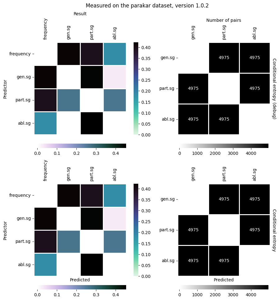
The most important is the heatmap: a matrix that shows how well each cell predicts each other cell. The higher the value, the darker the colour and vice-versa:

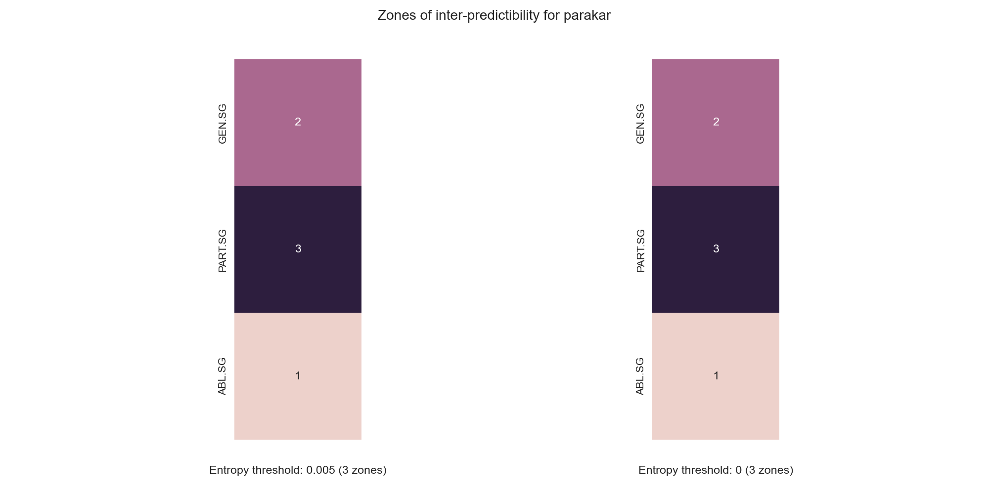
Qumin also tries to identify zones of interpredictability, that is sets of cells that are completely interpredictable. Our dataset, does not contain such cells:

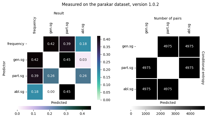
To fine-tune these plots, you can rerun the algorithm on pre-computed entropies with the following command: .. Here, the heatmap.annotate keyword asks to add the numeric results to the heatmap:

qumin action=ent_heatmap data=parakar/parakar.package.json \
pred.importResults=results/entropies/metadata.json \
hydra.run.dir=results/heatmaps heatmap.annotate=True

And the result:

Tip

Have a look at the heatmap reference to see all available options for entropy visualizations.